Recurrent Neural Networks and the Secrets of Sequence Learning

From music generation to predictive text and financial forecasting, deep learning has found its way into the world of sequences, and at the heart of this revolution lies a powerful architecture: Recurrent Neural Networks. Unlike traditional neural networks that see the world one snapshot at a time, RNNs remember the past, making them uniquely suited to understanding time, language, and structure in data. In this article, we’ll dive into how they work, where they shine, and why they’re both brilliant and flawed. If you’ve ever wondered how machines understand speech, translate languages, or even write poetry, you’re about to find out.

In this article:

1. What Are Recurrent Neural Networks?
2. How RNNs Work: The Power of Memory
3. Applications of RNNs in the Real World
4. The Problem of Vanishing Gradients (and the RNN’s Dark Side)
5. LSTMs and GRUs: Smarter Variants of the RNN
6. From RNNs to Transformers: A Shift in Sequence Modeling
7. References

1. What Are Recurrent Neural Networks?

In the world of deep learning, most models process data under the assumption that each input is independent of the next. This approach works well for tasks like image classification, where the structure of one image has little to do with another. But what about data that comes in sequences — like sentences, time series, or audio streams — where order matters and context is everything?

That’s where Recurrent Neural Networks (RNNs) come in. Unlike traditional feedforward neural networks that pass information in a single direction from input to output, RNNs are designed to recognize patterns across time by maintaining a memory of what they’ve seen so far.

At their core, RNNs are built on the idea of loops — they take an input, process it, and then feed a portion of their output back into themselves to influence future predictions. This recursive structure allows the network to retain information about previous elements in a sequence, making it especially powerful for tasks like:

• Predicting the next word in a sentence
• Analyzing stock price movements over time
• Translating language from one form to another
• Generating music or speech

🧠 Memory Through Hidden States

The key innovation of RNNs lies in what’s called the hidden state — a vector of numbers that gets updated at each step of the sequence. This hidden state acts as a sort of internal memory, capturing essential information about the sequence so far.

Mathematically, for each time step t, the RNN updates its hidden state h_t based on the current input x_t and the previous hidden state h_{t-1}:

cppCopiarEditarh_t = f(W_x * x_t + W_h * h_{t-1} + b)

Where:

• W_x and W_h are weight matrices,
• b is a bias vector, and
• f() is usually a nonlinear activation function like tanh or ReLU.

This formulation enables the model to “remember” previous inputs and use that information to influence its current output — a major step toward temporal reasoning in machines.

🔧 Practical Example: Predicting a Simple Sequence Using an RNN (Keras)

Let’s say we want to train a neural network to predict the next number in a sequence like:

csharpCopiarEditar[1, 2, 3] → 4  
[2, 3, 4] → 5  
[3, 4, 5] → 6  
...

This is a very basic case of sequence learning, but it’s perfect to illustrate how an RNN processes temporal dependencies.

🛠️ Step-by-step Code Using Keras (TensorFlow)

pythonCopiarEditarimport numpy as np
from tensorflow.keras.models import Sequential
from tensorflow.keras.layers import SimpleRNN, Dense

# Step 1: Prepare the data
X = []
y = []

# Create sequences like [1, 2, 3] -> 4
for i in range(1, 100):
    X.append([i, i+1, i+2])
    y.append(i+3)

# Convert to NumPy arrays and reshape for RNN input (samples, timesteps, features)
X = np.array(X)
y = np.array(y)
X = X.reshape((X.shape[0], X.shape[1], 1))  # 3 time steps, 1 feature each

# Step 2: Build the model
model = Sequential()
model.add(SimpleRNN(10, activation='relu', input_shape=(3, 1)))
model.add(Dense(1))
model.compile(optimizer='adam', loss='mse')

# Step 3: Train the model
model.fit(X, y, epochs=200, verbose=0)

# Step 4: Make a prediction
test_sequence = np.array([[98, 99, 100]])
test_sequence = test_sequence.reshape((1, 3, 1))
predicted = model.predict(test_sequence, verbose=0)
print(f"Predicted next number after [98, 99, 100]: {predicted[0][0]:.2f}")

✅ Output Example

bashCopiarEditarPredicted next number after [98, 99, 100]: 101.01

---

🧩 What This Teaches

This mini-project shows how a Recurrent Neural Network can:

• Take a sequence of inputs (timesteps),
• Learn the relationship between them,
• Predict the next value in the sequence by “remembering” the previous steps.

Even though this example uses numerical patterns (which are easy to model), the same principle applies to words in sentences, audio signals, and stock prices.

2. How RNNs Work: The Power of Memory

At the heart of Recurrent Neural Networks lies a key innovation that sets them apart from traditional neural architectures: memory.

In standard feedforward neural networks, the assumption is that all inputs are independent. While this works for tasks like image recognition, it falls short when context matters — like in language, music, or financial time series. RNNs were designed specifically to handle this challenge, by retaining and using information from previous inputs to influence the current output.

But how exactly does this “memory” work?

🔄 Step-by-Step: The Recurrent Mechanism

RNNs process input data sequentially, one time step at a time. At each time step t, the network receives:

• An input vector xₜ,
• The hidden state from the previous time step hₜ₋₁.

Using these two, it computes:

1. A new hidden state hₜ, and
2. An output yₜ (optional, depending on the task).

📐 The Mathematical Intuition

Let’s simplify the process using the following equations:

textCopiarEditarhₜ = tanh(Wₓ · xₜ + Wₕ · hₜ₋₁ + bₕ)
yₜ = Wᵧ · hₜ + bᵧ

Where:

• Wₓ, Wₕ, and Wᵧ are weight matrices,
• bₕ and bᵧ are bias vectors,
• tanh is the activation function (others like ReLU or sigmoid may also be used),
• hₜ is the updated hidden state (the network’s memory),
• yₜ is the output at time step t.

This recursive structure allows information to flow forward in time, as the hidden state evolves with each input. The network “remembers” useful patterns while forgetting irrelevant noise.

---

🧭 Why This Memory Matters

Let’s look at two concrete examples to appreciate the power of memory:

🔤 1. Language Modeling

In a sentence like:

“The cat sat on the mat.”

The word “mat” is predictable because of the context created by the previous words. An RNN, by remembering “The cat sat on the”, is able to generate or predict a logical continuation.

📉 2. Time Series Forecasting

In stock price prediction, recent prices influence the next price point. An RNN can learn temporal patterns like trends and seasonality because it carries the historical context from one timestep to the next.

---

⚠️ But Memory Has Its Limits…

One important caveat: basic RNNs struggle with long-term dependencies.

As the sequence grows, the influence of older inputs fades due to a problem known as the vanishing gradient. During training, small gradients backpropagated through many time steps can become too small to update earlier layers effectively. This means the model might forget relevant information from the distant past.

This limitation led to the development of more advanced RNN architectures like LSTM (Long Short-Term Memory) and GRU (Gated Recurrent Unit) — which you’ll learn about in a later chapter.

---

🎯 Summary

RNNs are powerful because they bring memory into machine learning. By keeping track of prior inputs through a hidden state, they learn to identify patterns over time — something essential for any task involving sequences. However, their memory isn’t perfect, and understanding its limits is crucial for designing effective models.

3. Applications of RNNs in the Real World

Recurrent Neural Networks (RNNs) have earned their place at the heart of some of the most impressive advancements in artificial intelligence, particularly in tasks where context and order matter. Unlike traditional feedforward networks, RNNs are designed to process sequential data, making them uniquely equipped to tackle problems where information unfolds over time. Let’s explore how this capability translates into real-world impact across different industries.

3.1 Natural Language Processing (NLP)

One of the most prominent domains where RNNs shine is natural language processing. Their ability to model the temporal structure of text has made them instrumental in:

• Text generation: Producing coherent sentences by predicting the next word based on previous input (e.g., chatbots and story generation).
• Machine translation: Translating text from one language to another by preserving word order and grammatical structure (e.g., Google Translate’s early RNN-based models).
• Speech recognition: Converting spoken language into text, where each word and syllable depends on what comes before it.

Even though architectures like Transformers have surpassed RNNs in many benchmarks, RNNs laid the groundwork and are still used in smaller or more resource-constrained applications.

3.2 Time Series Forecasting

Whether predicting stock prices, weather patterns, or sensor data, RNNs are valuable because they naturally handle temporal dependencies:

• Finance: Analysts use RNNs to model market trends and anticipate future asset movements.
• IoT and Smart Homes: RNNs can detect anomalies in time-series sensor data (e.g., identifying equipment failure).
• Energy usage prediction: Modeling energy consumption patterns based on historical usage.

Their memory of past inputs allows RNNs to make informed forecasts based on trends, seasonality, and previous behavior.

3.3 Healthcare and Biomedical Applications

In healthcare, sequential data is everywhere — from patient monitoring to genetic sequencing. RNNs have enabled:

• ECG anomaly detection: Identifying arrhythmias from heartbeat sequences.
• Electronic health record modeling: Predicting patient diagnoses or future hospital admissions.
• Drug discovery: Analyzing sequences of molecular structures for potential pharmaceutical candidates.

These applications are especially impactful in preventive medicine and patient risk modeling.

3.4 Music and Audio Generation

Just as in text, sequences matter in music. RNNs have been trained to:

• Generate original compositions that follow harmonic and rhythmic patterns.
• Predict musical notes in a melody or accompaniment.
• Analyze audio signals for tasks like genre classification or instrument recognition.

Notable examples include OpenAI’s early MuseNet experiments and projects like Google’s Magenta.

3.5 Video and Gesture Recognition

Video data is inherently sequential — a stream of images over time. RNNs help interpret this by:

• Recognizing gestures in motion sequences.
• Interpreting human activity from surveillance footage.
• Enhancing real-time human-computer interaction (e.g., virtual assistants that respond to body language).

These applications bridge AI with real-time human perception and behavior tracking.

---

In summary, RNNs have found their way into a variety of real-world challenges where understanding sequences is vital. From predictive healthcare to interactive music, their ability to remember and respond to context has made them indispensable — even as newer architectures emerge.

🧪 Practical Example: Text Generation with RNN in Python

To better understand how RNNs are applied in real-world scenarios, let’s walk through a simple yet illustrative example: building a Recurrent Neural Network (RNN) to generate text based on a short set of training sentences. We’ll use Keras with TensorFlow to make this as accessible as possible.

---

🔧 Requirements

Before you begin, make sure you have TensorFlow installed:

bashCopiarEditarpip install tensorflow

---

📜 Complete Python Code

pythonCopiarEditarimport numpy as np
import tensorflow as tf
from tensorflow.keras.models import Sequential
from tensorflow.keras.layers import Dense, SimpleRNN, Embedding
from tensorflow.keras.preprocessing.sequence import pad_sequences
from tensorflow.keras.preprocessing.text import Tokenizer

# Simple training corpus
corpus = [
    "machine learning is powerful",
    "deep learning drives innovation",
    "recurrent neural networks learn sequences",
    "neural networks are inspired by the brain",
    "artificial intelligence is the future"
]

# Tokenize the corpus
tokenizer = Tokenizer()
tokenizer.fit_on_texts(corpus)
total_words = len(tokenizer.word_index) + 1

# Create input sequences for n-gram training
input_sequences = []
for line in corpus:
    token_list = tokenizer.texts_to_sequences([line])[0]
    for i in range(1, len(token_list)):
        n_gram_sequence = token_list[:i+1]
        input_sequences.append(n_gram_sequence)

# Pad sequences
max_sequence_len = max([len(seq) for seq in input_sequences])
input_sequences = np.array(pad_sequences(input_sequences, maxlen=max_sequence_len, padding='pre'))

# Split into predictors (X) and label (y)
X = input_sequences[:, :-1]
y = tf.keras.utils.to_categorical(input_sequences[:, -1], num_classes=total_words)

# Define a simple RNN model
model = Sequential([
    Embedding(input_dim=total_words, output_dim=10, input_length=max_sequence_len - 1),
    SimpleRNN(units=64),
    Dense(total_words, activation='softmax')
])

model.compile(loss='categorical_crossentropy', optimizer='adam', metrics=['accuracy'])
model.summary()

# Train the model
model.fit(X, y, epochs=200, verbose=0)

# Function to generate new text
def generate_text(seed_text, next_words=5):
    for _ in range(next_words):
        token_list = tokenizer.texts_to_sequences([seed_text])[0]
        token_list = pad_sequences([token_list], maxlen=max_sequence_len - 1, padding='pre')
        predicted = np.argmax(model.predict(token_list, verbose=0), axis=-1)
        output_word = ""
        for word, index in tokenizer.word_index.items():
            if index == predicted:
                output_word = word
                break
        seed_text += " " + output_word
    return seed_text

# Test the model
print(generate_text("neural networks", next_words=5))

---

🧠 What’s Happening Here?

• The model learns to predict the next word in a sequence from very short example sentences.
• It uses an Embedding layer to map words into vector space and a SimpleRNN layer to process sequences.
• Once trained, it can generate new phrases by continuing a seed sentence such as "neural networks".

---

📌 Example Output

plaintextCopiarEditarneural networks learn sequences are inspired by

Keep in mind, the generated text depends on the quality and size of the training data.

---

🧭 Where to Go From Here?

• Replace the SimpleRNN layer with more powerful alternatives like LSTM or GRU.
• Train the model on larger and more complex datasets (e.g., books, news articles, or code).
• Add temperature sampling to make the generated text more diverse.

4. The Problem of Vanishing Gradients (and the RNN’s Dark Side)

Recurrent Neural Networks (RNNs) opened new doors in the world of machine learning by allowing models to learn from sequences — not just from fixed-size inputs. However, this power comes with a price. Like many innovations, RNNs have their own “dark side.” One of the most well-known and persistent issues they face is the vanishing gradient problem — a mathematical roadblock that can limit their ability to learn long-term dependencies.

In this chapter, we’ll explore:

• What the vanishing gradient problem is.
• Why RNNs are particularly vulnerable to it.
• How it affects training performance.
• What strategies and architectures were developed to overcome it.

---

🔁 Backpropagation Through Time (BPTT)

To understand the vanishing gradient issue, we first need to revisit how RNNs learn.

RNNs are trained using a special version of backpropagation called Backpropagation Through Time (BPTT). Because RNNs unfold over time, they’re essentially a deep network where each “layer” represents the network at a specific time step. When training, the gradients (i.e., error signals used to update weights) are passed backward through each time step to adjust the weights.

This backward pass accumulates the chain rule of derivatives across many time steps:

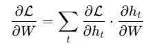
The deeper (or longer) the sequence, the more steps this chain must traverse. And that’s where problems begin.

---

🧨 What Is the Vanishing Gradient Problem?

The vanishing gradient problem occurs when the gradients — small values used to update the model’s weights — shrink rapidly as they are propagated backward through many layers (or time steps).

In simpler terms:

• Early layers (or time steps) receive extremely small updates.
• These small updates are often rounded to zero by the computer.
• As a result, the model “forgets” how to learn from earlier parts of the sequence.

Mathematically, it arises from repeated multiplication of small values (i.e., derivatives of activation functions like tanh or sigmoid), which can shrink exponentially:

​​

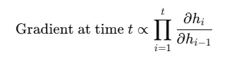
If each of those partial derivatives is less than 1, the product becomes smaller and smaller, eventually tending toward zero.

---

🧠 Why It Matters

The vanishing gradient problem limits an RNN’s ability to capture long-range dependencies. This is especially problematic for tasks like:

• Language modeling, where the meaning of a word might depend on something said 10 or 20 words earlier.
• Music generation, where the structure may span over dozens of time steps.
• Time series forecasting, where seasonal or long-term trends are critical.

As a result, basic RNNs often fail to learn meaningful patterns over long sequences, even when more training data is available.

---

⚠️ An Example in Practice

Let’s say you’re training an RNN to complete the sentence:

“If it rains tomorrow, I will take my _.”

The correct answer is likely “umbrella,” but that information depends on understanding the word “rains,” which occurred much earlier in the sentence. If the RNN suffers from vanishing gradients, it might forget “rains” entirely by the time it gets to “take my,” and fail to predict the correct word.

---

🛠 Solutions to the Vanishing Gradient Problem

Over time, researchers developed several clever solutions to address this issue:

1. Better Activation Functions

Functions like ReLU (Rectified Linear Unit) avoid saturation and help keep gradients from shrinking too quickly. However, standard RNNs using ReLU can still suffer from exploding gradients.

2. Gradient Clipping

This is a simple fix: if a gradient becomes too large or too small, we clip it to a maximum or minimum threshold. While helpful for training stability, it doesn’t eliminate the root cause.

3. Gated Architectures: LSTM and GRU

This is the game changer.

• LSTM (Long Short-Term Memory) networks introduce special structures called gates — input, forget, and output gates — that control the flow of information and protect against vanishing gradients.
• GRU (Gated Recurrent Unit) is a simpler alternative to LSTM but performs similarly in many applications.

These architectures are explicitly designed to maintain a constant error flow across long sequences. Instead of forgetting everything with tiny gradients, they retain information selectively, almost like short-term memory in the brain.

---

🔄 The Big Takeaway

The vanishing gradient problem is not a minor detail — it’s a fundamental limitation of vanilla RNNs. Understanding it helps explain why more sophisticated architectures like LSTM and GRU became the new standard for working with sequential data.

In the next chapter, we’ll explore these architectures in more depth and see how they address the limitations discussed here.

5. LSTMs and GRUs: Smarter Variants of the RNN

Recurrent Neural Networks (RNNs) changed how machines process sequences, but as we saw in the previous chapter, they face serious limitations—especially when trying to learn long-term dependencies due to the vanishing gradient problem. To address these issues, researchers introduced more sophisticated types of RNNs: Long Short-Term Memory (LSTM) networks and Gated Recurrent Units (GRU).

These architectures incorporate built-in mechanisms to regulate the flow of information, allowing them to “remember” relevant details for long periods and forget what’s not important. In this chapter, we’ll break down how these smarter variants work, why they perform better, and how to choose between them for your projects.

---

🧠 Why We Needed Something Smarter

Before diving into the mechanics, let’s remind ourselves of the key problem: basic RNNs struggle to preserve information over long sequences. They update their hidden state at every time step, meaning useful information from earlier inputs gets diluted or lost as the sequence grows.

The solution? Introduce gates—structures that help the network decide what to keep, what to update, and what to forget.

---

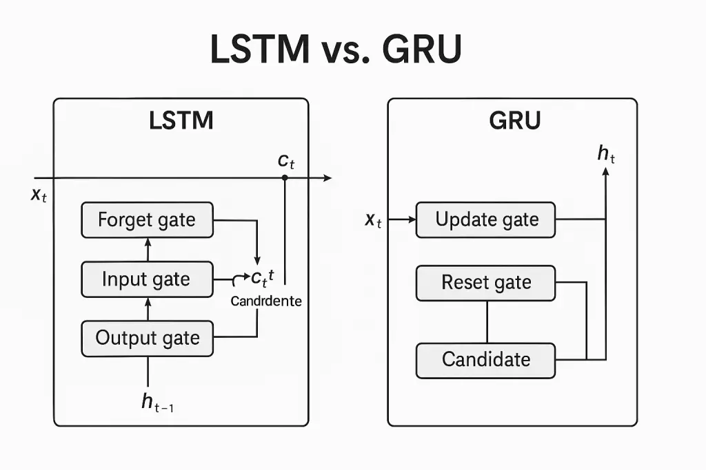
🔐 LSTM: Long Short-Term Memory

LSTMs were introduced by Hochreiter and Schmidhuber in 1997 to overcome RNNs’ shortcomings. What makes them special is the memory cell and three gates that control the information flow:

1. Forget Gate (f_t) – Decides what information to discard from the cell state.
2. Input Gate (i_t) – Decides what new information to store in the cell state.
3. Output Gate (o_t) – Determines what part of the cell state to output as the hidden state.

🧬 How It Works (Conceptually)

At each time step, the LSTM does the following:

• Looks at the current input and previous hidden state.
• Uses the forget gate to remove unneeded information from the memory cell.
• Uses the input gate to add relevant new information.
• Uses the output gate to pass forward what’s important.

This creates a persistent memory structure that learns what matters and for how long.

🧮 LSTM Equations (Simplified)

Let’s peek under the hood:

textCopiarEditarf_t = σ(W_f · [h_{t-1}, x_t] + b_f)         # Forget gate
i_t = σ(W_i · [h_{t-1}, x_t] + b_i)         # Input gate
c̃_t = tanh(W_c · [h_{t-1}, x_t] + b_c)      # Candidate values
c_t = f_t * c_{t-1} + i_t * c̃_t             # New cell state
o_t = σ(W_o · [h_{t-1}, x_t] + b_o)         # Output gate
h_t = o_t * tanh(c_t)                        # New hidden state

Here, σ is the sigmoid function, and tanh squashes values between -1 and 1. The memory cell c_t acts like a conveyor belt of relevant information, selectively modified as needed.

---

⚡ GRU: Gated Recurrent Unit

Introduced in 2014 by Cho et al., the GRU is a simpler, faster alternative to LSTM. It merges the forget and input gates into a single update gate and eliminates the separate cell state—everything happens within the hidden state.

GRU Gates

1. Update Gate (z_t) – Controls how much of the past information to keep.
2. Reset Gate (r_t) – Decides how much past information to forget when computing the new candidate state.

GRU Equations

textCopiarEditarz_t = σ(W_z · [h_{t-1}, x_t])               # Update gate
r_t = σ(W_r · [h_{t-1}, x_t])               # Reset gate
h̃_t = tanh(W · [r_t * h_{t-1}, x_t])        # Candidate activation
h_t = (1 - z_t) * h_{t-1} + z_t * h̃_t       # Final hidden state

GRUs are computationally more efficient and often perform just as well as LSTMs, especially on smaller datasets.

---

🧪 LSTM vs GRU: How to Choose

Feature	LSTM	GRU
Number of Gates	3 (forget, input, output)	2 (update, reset)
Memory Cell	Yes	No (hidden state only)
Computational Cost	Higher	Lower
Training Speed	Slower	Faster
Performance	Better on complex tasks	Often similar, sometimes better on smaller datasets

If you’re just starting out or need speed, GRUs are a great choice. For more complex tasks with longer dependencies, LSTMs may yield better results.

---

🚀 Real-World Success Stories

• Speech Recognition: Google’s voice search used LSTMs to improve accuracy.
• Language Translation: GRUs were used in early versions of neural machine translation systems.
• Chatbots: LSTMs are often employed in sequence-to-sequence models for conversational agents.
• Finance: Both LSTMs and GRUs are used to predict stock prices or detect anomalies in financial time series.

---

🧩 Summary

LSTMs and GRUs are evolutionary steps that solved key issues with vanilla RNNs by introducing smart memory mechanisms. Their gating systems make them capable of learning long-term dependencies, which is essential for most real-world sequence modeling tasks.

In the final chapter, we’ll explore how you can put these models into practice using popular Python libraries like TensorFlow and PyTorch, and share tips to get started on your own sequence learning project.

6. From RNNs to Transformers: A Shift in Sequence Modeling

As effective and groundbreaking as Recurrent Neural Networks (RNNs) have been, they are no longer the only game in town. In recent years, the field of deep learning has witnessed a paradigm shift with the emergence of Transformers — a new class of architectures that is revolutionizing sequence modeling.

RNNs, including LSTMs and GRUs, process sequences step by step, maintaining a hidden state that carries information across time. This sequential nature, however, comes with a cost: it limits parallelization, which slows down training. It also makes long-range dependencies more difficult to capture, despite improvements like gating mechanisms.

Transformers, first introduced in the seminal paper “Attention Is All You Need” (Vaswani et al., 2017), take a radically different approach. Instead of processing inputs sequentially, Transformers use self-attention mechanisms to capture dependencies across an entire sequence simultaneously. This allows for:

• Greater parallelization, making training significantly faster.
• Better handling of long-term dependencies, without the vanishing gradient issues.
• Scalability, enabling massive pretraining on large datasets (e.g., GPT, BERT).

Where RNNs see text as a chain of steps, Transformers view it as a global context to be interpreted all at once. This shift has propelled the development of state-of-the-art language models and has extended into other domains such as vision, audio, and even protein folding.

Still, RNNs maintain their relevance in many domains, especially where training efficiency and lower data requirements are crucial. Understanding RNNs and their successors is essential for anyone exploring sequence-based learning problems, from time series forecasting to conversational AI.

7. References

• Hochreiter, S., & Schmidhuber, J. (1997). Long Short-Term Memory. Neural Computation, 9(8), 1735–1780.
• Cho, K., van Merriënboer, B., Gulcehre, C., Bahdanau, D., Bougares, F., Schwenk, H., & Bengio, Y. (2014). Learning Phrase Representations using RNN Encoder–Decoder for Statistical Machine Translation. arXiv preprint arXiv:1406.1078.
• Vaswani, A., Shazeer, N., Parmar, N., Uszkoreit, J., Jones, L., Gomez, A. N., … & Polosukhin, I. (2017). Attention is All You Need. Advances in Neural Information Processing Systems, 30.
• Goodfellow, I., Bengio, Y., & Courville, A. (2016). Deep Learning. MIT Press.
• Chollet, F. (2021). Deep Learning with Python (2nd ed.). Manning Publications.
• Brownlee, J. (2017). Introduction to Time Series Forecasting with Python: How to Prepare Data and Develop Models to Predict the Future. Machine Learning Mastery.
• Olah, C. (2015). Understanding LSTM Networks. https://colah.github.io/posts/2015-08-Understanding-LSTMs/
• TensorFlow Documentation – https://www.tensorflow.org
• PyTorch Documentation – https://pytorch.org

Disclaimer

This article was written with the support of AI tools to assist in the generation, organization, and refinement of content. While it reflects careful research and editorial oversight, readers are encouraged to consult the listed references and conduct further study for a deeper understanding.