In the expansive landscape of computer networking and artificial intelligence (AI), several concepts stand out as the linchpins of computational processing, underpinning the very essence of intelligent automation. One such concept, often perceived as an enigma by budding computer scientists and established professionals alike, is the Finite State Machine (FSM). As our world gravitates more towards interconnected systems and AI-driven solutions, understanding FSMs is no longer an optional luxury—it’s a necessity.
In this article:
- What is a Finite State Machine?
- Types of Finite State Machines
- FSMs in Protocol Design
- Designing an FSM: A Step-by-Step Guide
- Finite State Machines vs. Turing Machines
- Conclusion
The convergence of traditional computer networking with the burgeoning field of AI has led to an era where concepts like FSMs serve as bridges, linking fundamental networking practices with AI’s abstract theories. Let’s embark on a journey to decipher this vital component, illuminating its role, significance, and intricacies in today’s technologically driven world.
Chapter 1: What is a Finite State Machine?
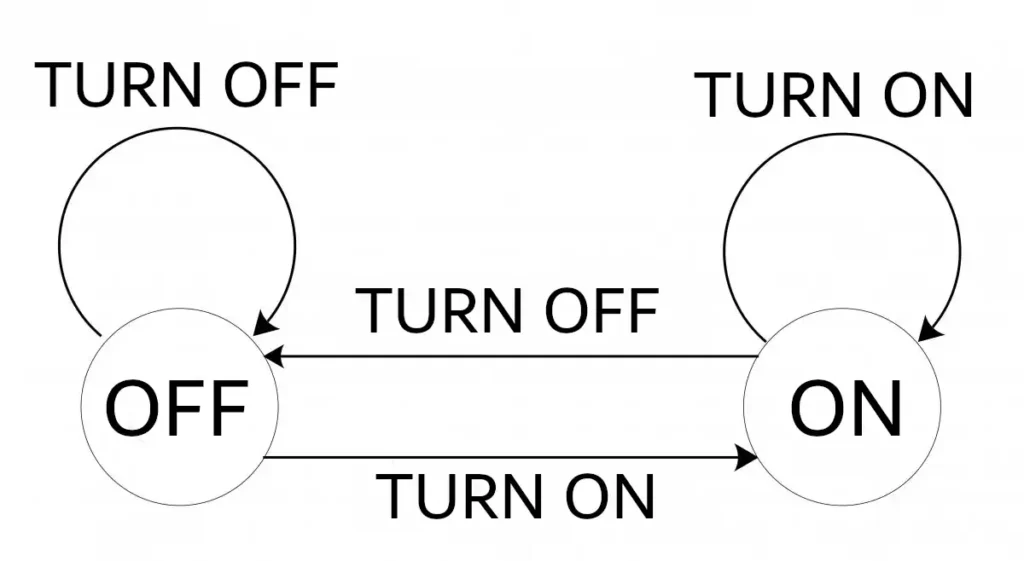
At its core, a Finite State Machine is a mathematical model of computation, representing a system that can exist in only one state at a given time. It’s akin to a systematic roadmap where each point, or state, leads to another based on predetermined conditions. These machines serve to respond to a series of inputs, transitioning between states and producing outputs based on those inputs and the machine’s set rules.
Picture a vending machine: you insert a coin, and the machine transitions from a “waiting for coin” state to an “awaiting selection” state. Once you make a selection, it moves to the “dispensing” state, and so forth. Each state transition depends on the input (your actions) and the machine’s set conditions (prices, available items). This simplistic analogy encapsulates the essence of FSMs, which, in the world of computer networking and AI, take on much more complex, abstract roles. Their deterministic nature allows for predictability, making them invaluable in scenarios requiring sequential logic, like protocol developments or natural language processing in AI.
» To read next: Quality of Service (QoS) Definition!
Chapter 2: Types of Finite State Machines
In the vast realm of computational systems, understanding the nuanced differences between various Finite State Machines (FSMs) is crucial. Broadly, FSMs are bifurcated into two primary categories: Deterministic Finite State Machines (DFSMs) and Non-deterministic Finite State Machines (NFSMs). Let’s delve into each type, understanding their structure, functionality, and intrinsic differences.
Deterministic Finite State Machines (DFSMs):
A deterministic FSM is characterized by its ability to determine its next state based solely on its current state and the input it receives. There’s a distinct predictability in its transition. For every state and every input symbol, there’s one and only one transition to a next state.
Consider, for instance, a digital lock system. Based on the current state (locked/unlocked) and the input (correct code entry), the system determines the next state, either remaining locked or transitioning to unlocked. No ambiguity exists.
Non-deterministic Finite State Machines (NFSMs):
In stark contrast, an NFSM might have zero, one, or multiple transitions from one state for a particular input. Its non-deterministic nature doesn’t imply randomness but rather denotes multiple possible future outcomes. An NFSM can transition to any combination of states in its set. Hence, from any given state, it can move to multiple next states based on a particular input.
Imagine a game scenario where a player’s move can lead to multiple potential next steps. Depending on the input, the game can transition into various potential scenarios, making its behavior inherently non-deterministic.
While DFSMs have a clear linear path of progression, NFSMs require more computational effort, especially when trying to determine acceptance of a particular input string. Interestingly, for every NFSM, there’s an equivalent DFSM. However, converting an NFSM to a DFSM might result in an exponential increase in the number of states.
» You may also like: What is Deep Learning?
Chapter 3: FSMs in Protocol Design
As communication networks burgeon, protocols—the rules that define data communication—become increasingly vital. These protocols ensure that information is correctly sent, received, and understood, even in intricate networks. Finite State Machines serve as the backbone in designing these protocols, enabling predictable reactions to various input combinations.
Role of FSMs in Protocol Development:
Each protocol defines a set of possible states, conditions that trigger a transition between states, and actions that result from state changes. FSMs depict these states and transitions graphically, assisting engineers in comprehending and designing complex communication protocols.
For example, the Transmission Control Protocol (TCP) is a cornerstone of Internet data exchange. TCP involves numerous states like “LISTEN,” “ESTABLISHED,” and “FIN_WAIT.” FSMs enable engineers to visualize the transition between these states, based on events like receiving a SYN (synchronize) packet or ACK (acknowledgment) packet.
FSMs in Error Detection and Recovery:
In data communication, errors are inevitable. FSMs help in both detecting these errors and ensuring successful data recovery. If a protocol transitions to an unexpected state, the FSM can flag this as an error. Subsequent recovery procedures, also managed by FSMs, then come into play to restore the integrity of the communication.
Handling Asynchronous Events:
In real-world scenarios, network events occur asynchronously. A protocol must handle diverse input sequences, which might occur simultaneously. FSMs, with their deterministic nature, are instrumental in managing such sequences. They ensure that the protocol reacts appropriately, even when bombarded with asynchronous events.
In conclusion, FSMs aren’t just theoretical constructs but practical tools that breathe life into network protocols. From ensuring seamless data communication to managing unforeseen network events, FSMs play an integral role in the world of computer networking, making them indispensable for any network engineer.
Chapter 4: Designing an FSM: A Step-by-Step Guide
Creating a Finite State Machine (FSM) is akin to crafting a story—a series of events lead to specific outcomes, depending on conditions and choices made. Here’s a step-by-step guide to conceptualizing and constructing a basic FSM:
1. Define the Purpose of Your Finite State Machine:
Before diving into design, clarify the FSM’s role. What computational or operational problem should it solve?
2. Identify States:
List all possible states the machine can be in. For a door lock system, states might include LOCKED and UNLOCKED.
3. Determine Inputs:
Identify the range of inputs the FSM will receive. For our door lock, inputs could be a KEY_INSERTED, CORRECT_CODE_ENTERED, or INCORRECT_CODE_ENTERED.
4. Map Transitions:
For each state, define how various inputs will cause transitions to other states. For instance, from LOCKED, the input CORRECT_CODE_ENTERED might transition the system to UNLOCKED.
5. Specify Outputs (if any):
Not all FSMs produce outputs, but if yours does, determine what each state transition results in. In our example, an output might be a light turning GREEN when the door unlocks.
6. Visualize with a Diagram:
Draw states as circles and transitions as arrows, creating a clear diagrammatic representation of your FSM.
7. Test Your FSM:
Once your FSM is designed, run through various input scenarios to ensure it behaves as expected. This helps identify any missing transitions or possible ambiguities.
Chapter 5: Finite State Machines vs. Turing Machines
In the universe of computation, both Finite State Machines (FSMs) and Turing Machines (TMs) hold pivotal roles. However, while they might seem similar, their computational capabilities differ dramatically.
Finite State Machines:
As detailed earlier, an FSM has a finite number of states and transitions between them based on inputs. It lacks memory about past inputs (beyond its current state). FSMs are deterministic (DFSM) or non-deterministic (NFSM) and are limited in their computational power.
Turing Machines:
A Turing Machine, named after the British mathematician Alan Turing, is a more powerful computational model. It consists of an infinite tape, a tape head that moves left or right, and a state machine. The tape stores input and auxiliary information, granting TMs memory capabilities.
Comparing Capabilities:
- Memory: FSMs have no “memory” beyond their current state. In contrast, TMs can use their tape to store and retrieve an unlimited amount of data, granting them superior computational flexibility.
- Computational Power: Every function that an FSM can compute can also be computed by a TM. However, there are functions a TM can compute that an FSM cannot, making TMs strictly more powerful.
- Universality: There exists a Universal Turing Machine that can simulate any other Turing Machine, making TMs programmable and versatile. No such universal model exists for FSMs.
- Decidability: While FSMs are limited and can’t solve undecidable problems, TMs can represent these problems even if they can’t always provide solutions.
Conclusion
The landscape of computational models is vast and varied. Finite State Machines, with their deterministic nature, are invaluable in scenarios requiring sequential logic, like protocol developments. Turing Machines, on the other hand, provide a broader computational canvas, encapsulating problems that stretch the boundaries of decidability.
As technology continues to evolve, the concepts behind these machines not only remain relevant but become ever more crucial, helping us navigate the complex tapestry of computational challenges and possibilities.
Further Reading
- “Finite State Machines and Algorithmic State Machines: Fast and Simple Design of Complex Finite State Machines“, by Samary Baranov
- “Regular Algebra and Finite Machines“, by John Horton Conway
- “Finite State Machines in Hardware: Theory and Design (with VHDL and SystemVerilog) (The MIT Press)“, by Volnei A. Pedroni