In this article, we deeply address the topic of Network Infrastructure Design. We are going to study the computer networking issues that arise when planning a campus network. The term campus network applies to any network that has multiple LANs interconnected.
The LANs are located in multiple buildings close together and interconnected with switches and routers. So, here we are going to cover the planning and design of a very simple campus network that includes network design, IP subnetting, VLAN configuration, and routed network configuration.
In this article:
Physical Network Design
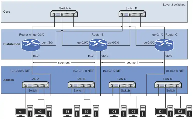
Most campus networks follow a design that has core, distribution, and access layers. These layers, shown in Image 1, can be spread out into more layers or compacted into fewer, depending on the size of these networks. This three-layer network structure is incorporated in campus networks to improve data handling and routing within the network.
Core
The network core typically contains routers or high-end Layer 3 switches. The core is the backbone of the network. The major percentage of a network’s data traffic flows through the core. The core must be able to rapidly forward data to other portions of the network. Data congestion, if possible, should be avoided at the core. This means that unnecessary route policies should be avoided. An example of a route policy is traffic filtering, which limits what traffic can pass from one part of a network to another. Be aware that it takes time for a router to inspect each data packet, and superfluous route policies can slow down the network’s data traffic.
“CORE LAYER: the Backbone of the Network”
High-end Layer 3 switches and routers are normally selected for use in the core. Of the two, the Layer 3 switch is by far the best choice. A Layer 3 switch is basically a router that uses hardware instead of software to make routing choices. The advantage of the Layer 3 switch is the speed at which it can make a routing choice and establish a network connection.
Using Layer 2 switch
Four budget reasons, we can choose another alternative for networking hardware in the core, that is a Layer 2 switch. The Layer 2 switch does not make any routing decisions and can quickly make network connection decisions based on the network hardware connected to its ports. The advantage of using the Layer 2 switch in the core is cost. The disadvantage is that the Layer 2 switch does not route data packets; however, high-speed Layer 2 switches are more affordable than high-speed routers and Layer 3 switches.
Redundancy
A vital design issue in a campus network and the core is redundancy. Redundancy provides for a backup route or network connection in case of a link failure. The core hardware is typically interconnected to all distribution network hardware, as shown in Image 1 (above). The goal is to ensure that data traffic continues, even if a core networking device or link fails.
Distribution Layer
The distribution layer in the network is the point where the individual LANs connect to the campus network routers or Layer 3 switches. Routing and filtering policies are more easily implemented at the distribution layer without having a negative impact on the performance of the network data traffic. Also, the speed of the network data connections at the distribution layer is naturally slower than at the core.
For example, connection speeds at the core should be the highest possible, such as 1 or 10 gigabits, where the data speed connections at the distribution layer could be 100 Mbps or 1 gigabit. Image 1 (above) shows the connections to the access and core layers via the router’s Ethernet interfaces.
Each layer beyond the core breaks the network into smaller networks with the final result being a group of networks that are capable of handling the amount of traffic generated. The design should thus incorporate some level of redundancy.
“DISTRIBUTION LAYER: point where the individual LAN’s connect together”
Access Layer
The access layer is where the networking devices in a LAN connect together. The network hardware used here is typically a Layer 2 switch. A switch is a better choice because it forwards data packets directly to destination hosts connected to its ports, and network data traffic is not forwarded to all hosts in the network. The exception to this is a broadcast where data packets are sent to all hosts connected to the switch.
“ACCESS LAYER: where the networking devices in a LAN connect together”
Data Flow
Another important networking topic is how data traffic flows in the core, distribution, and access layers of a campus LAN. In reference to Image 1, if computer A1 in LAN A sends data to computer D1 in LAN D, the data is first sent through the switch in LAN A and then to Router A in the distribution layer. Router A then forwards the data to the core switches, Switch A or Switch B. Switch A or Switch B then forwards the data to Router C. The data packet is then sent to the destination host in LAN D.
Here are some questions frequently asked when setting up a network that implements the core, distribution, and access layers:
• In what layer are the campus network servers (web, email, DHCP, DNS, and so on) located? This varies for all campus networks, and there is not a definitive answer. However, most campus network servers are located in the access layer.
• Why not connect directly from Router A to Router C at the distribution layer? There are network stability issues when routing large amounts of network data traffic if the networks are fully or even partially meshed together. This means that connecting routers together in the distribution layer should be avoided.
• Where is the campus backbone located in the layers of a campus network? The backbone of a campus network carries the bulk of the routed data traffic. Based on this, the backbone of the campus network connects the distribution and the core layer networking devices.
Selecting the Media
This is what you have to consider when choosing the media to use to interconnect networks in a campus network: Desired data speed, Distance for connections and Budget
Desired data speed
The desired data speed for the network connection is probably the first consideration given when selecting the network media. Twisted-pair cable works well at 100 Mbps and 1 Gbps and is specified to support data speeds of 10-gigabit data traffic. Fiber-optic cable supports LAN data rates up to 10 Gbps or higher. Wireless networks support data rates up to 200+ Mbps.
Distance
The distance consideration limits the choice of media. CAT 6/5e or better have a distance limitation of 100 meters. Fiber-optic cable can be run for many kilometers, depending on the electronics and optical devices used. Wireless LAN connections can also be used to interconnect networks a few kilometers apart.
Budget
The available budget is always the final deciding factor when planning the design for a campus LAN. If the budget allows, fiber-optic cable is probably the best overall choice, especially in the high-speed backbone of the campus network. The cost of fiber is continually dropping, making it more competitive with lower-cost network media, such as twisted-pair cable. Also, fiber cable will always be able to carry a greater amount of data traffic and can easily grow with the bandwidth requirements of a network.
Twisted-pair cable is a popular choice for connecting computers in a wired LAN. The twisted-pair technologies support bandwidths suitable for most LANs, and the performance capabilities of twisted-pair cable is always improving.
Wireless LANs are being used to connect networking devices together in LANs where a wired connection is not feasible or mobility is the major concern. For example, a wireless LAN could be used to connect two LANs in a building together. This is a cost-effective choice if there is not a cable duct to run the cable to interconnect the LANs or if the cost of running the cable is too high. Also, wireless connections are playing an important role with mobile users within a LAN. The mobile user can make a network connection without having to use a physical connection or jack. For example, a wireless LAN could be used to enable network users to connect their mobile computers to the campus network.
IP Subnet Design
Once the physical infrastructure for a network is in place, the next big step is to plan and allocate IP space for the network. Take time to plan the IP subnet design, because it is not easy to change the IP subnet assignments once they are in place. It is crucial for a network engineer to consider three factors before coming up with the final IP subnet design. These three factors are
1. The assigned IP address range
2. The number of subnetworks needed for the network
3. The size or the number of IP host addresses needed for the network
The final step in designing the IP subnet is to assign an IP address to the interface that will serve as the gateway out of each subnet.
IP Address Range
The IP address range defines the size of the IP network you can work with. In some cases, a classless interdomain routing (CIDR) block of public IP addresses might be allocated to the network by an ISP. For example, the block of IP address 206.206.156.0/24 could be assigned to the network. This case allocates 256 IP addresses to the 206.206.156.0 network. In another case, a CIDR block of private IP addresses, like 10.10.10.0/24, could be used. In this case, 256 IP addresses are assigned to the 10.10.10.0 network. For established networks with an IP address range already in use, the network engineer generally has to work within the existing IP address assignments. With a brand-new network, the engineer has the luxury of creating a network from scratch.
In most network situations, an IP address block will have been previously assigned to the network for Internet use. The public IP addresses are typically obtained from the ISP (Internet service provider). This IP block of addresses could be from Class A, B, or C networks, as shown in Table 1.
| Class | Address Range |
| Class A | 0.0.0.0 to 127.255.255.255 |
| Class B | 128.0.0.0 to 191.255.255.255 |
| Class C | 192.0.0.0 to 223.255.255.255 |
Today, only public Class C addresses are assigned by ISPs (Internet Service Providers), and most of them are not even a full set of Class C addresses (256 IP addresses). A lot of ISPs partition their allotted IP space into smaller subnets and then, in turn, provide those smaller portions to the customers. The bottom line is the limited number of public IP addresses are now a commodity on the Internet, and it is important to note that there are fees associated with acquiring an IP range from an ISP.
Not many institutions or businesses have the luxury of using public IP addresses inside their network anymore. This is because the growing number of devices being used in a network exceeds the number of public IP addresses assigned to them. The solution is that most networks are using private IP addresses in their internal network. Private addresses are IP addresses set aside for use in private intranets. An intranet is an internal internetwork that provides file and resource sharing. Private addresses are not valid addresses for Internet use, because they have been reserved for internal use and are not routable on the Internet. However, these addresses can be used within a private LAN (intranet) to create the internal IP network.
Private IP Addresses
The private IP addresses must be translated to public IP addresses using techniques like NAT (Network Address Translation) or PAT (Port Address Translation) before being routed over the Internet. For example, computer 1 in the home network (see Image 2) might be trying to establish a connection to an Internet website. The wireless router uses NAT to translate computer 1’s private IP address to the public IP address assigned to the router. The router uses a technique called overloading, where NAT translates the home network’s private IP addresses to the single public IP address assigned by the ISP. In addition, the NAT process tracks a port number for the connection. This technique is called Port Address Translation (PAT).
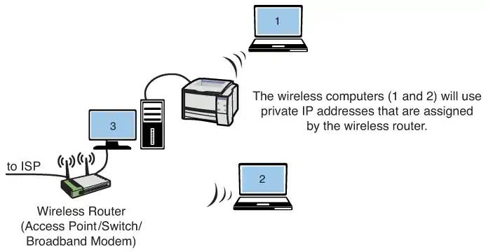
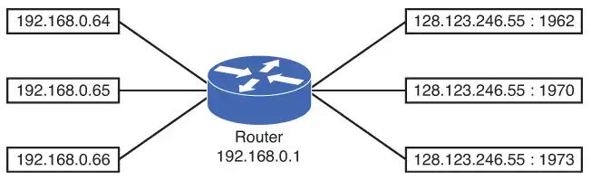
The router stores the home network’s IP address and port number in a NAT lookup table. The port number differentiates the computer that is establishing a connection to the Internet because the router uses the same public address for all computers. This port number is used when a data packet is returned to the home network. This port number identifies the computer that established the Internet connection, and the router can deliver the data packet back to the correct computer. An example of this conversion is provided in Image 3.
This example shows three data connections originating from the home network of 192.168.0.0/24. A single 128.123.246.55 IP address is used for the Internet connection. Port address translation is being used to map the data packet back to the origination source. In this case, the port numbers are 1962, 1970, and 1973.
Determining the Number of Subnetworks Needed for the Network
The use of private IP addresses is a viable technique for creating a large amount of IP addresses for intranet use. Obviously, there is a big difference when designing an IP network for a single network than there is when designing an IP network for multiple networks. When designing an IP network for one single network, things are quite simple. This type of configuration is typically found in the home, small office, or a small business environment where one IP subnet is allocated and only one small router is involved.
For situations requiring multiple networks, each network must be sized accordingly. Therefore, the subnet must be carefully designed. In addition, networks with multiple subnets require a router or multiple routers with multiple routed network interfaces to interconnect the networks. For example, if the network engineer is using private addresses and needs to design for three different networks, one possibility is to assign 10.10.10.0/24 for the first network, 172.16.0.0/24 for the second network, and 192.168.1.0/24 for the third network. Is this a good approach? Technically, this can be done, but it is probably not logically sound.
It makes more sense to group these networks within the same big CIDR block. This will make it easier for a network engineer to remember the IP assignments and to manage the subnets. A better design is to assign 10.10.10.0/24 to the first network, 10.10.20.0/24 to the second network, and 10.10.30.0/24 to the third network.
All three networks are all in the same “10” network, which makes it easier for the network engineer to track the IP assignments. The term subnet and network are used interchangeably in multiple network environments. The term subnet usually indicates a bigger network address is partitioned and is assigned to smaller networks or subnets.
Another design factor that the network engineer must address is the network size. Two questions that a good network engineer must ask are
• How many network devices must be accommodated in the network? (Current demand)
• How many network devices must be accommodated in the future? (Future growth)
Simply put, the IP network must be designed to accommodate the current demand, and it must be designed to accommodate future growth. Once the size of a network is determined, a subnet can be assigned. In the case of a single network, the design is not too complicated. For example, if the network needs to be able to accommodate 150 network devices, an entire Class C address, like 192.168.1.0/24, can be assigned to the network.
This will handle the current 150 network devices and leave enough room for growth. In this example, 104 additional IP address will be available for future growth.
When allocating IP address blocks, a table like Table 2 can be used to provide the CIDR for the most common subnet masks and their corresponding number of available IP addresses.
Table 2. CIDR—Subnet Mask-IPs Conversion
| CIDR | Subnet Mask | IPs |
| /16 | 255.255.0.0 | 65534 |
| /17 | 255.255.128.0 | 32768 |
| /18 | 255.255.192.0 | 16384 |
| /19 | 255.255.224.0 | 8192 |
| /20 | 255.255.240.0 | 4096 |
| /21 | 255.255.248.0 | 2048 |
| /22 | 255.255.252.0 | 1024 |
| /23 | 255.255.254.0 | 512 |
| /24 | 255.255.255.0 | 256 |
| /25 | 255.255.255.128 | 128 |
| /26 | 255.255.255.192 | 64 |
| /27 | 255.255.255.224 | 32 |
| /28 | 255.255.255.240 | 16 |
| /29 | 255.255.255.248 | 8 |
| /30 | 255.255.255.252 | 4 |
| /31 | 255.255.255.254 | 2 |
| /32 | 255.255.255.255 | 1 |
Even with a much smaller network, like the home network, where only a handful of network computers and peripherals are present, an entire Class C private address is generally allocated to the home network. In fact, most home routers are preconfigured with a private Class C address within the 192.168.0.0–192.168.0.255 range. This technique is user friendly and easy to use and sets aside private IP addresses for internal network use. This technique virtually guarantees that users will never have to worry about subnetting the CIDR block.
For a bigger network that must handle more than 254 network devices, a supernet can be deployed. A supernet is when two or more classful contiguous networks are grouped together. The technique of supernetting was proposed in 1992 to eliminate the class boundaries and make available the unused IP address space.
Supernet: Two or more classful contiguous networks are grouped together.
Supernetting allows multiple networks to be specified by one subnet mask. In other words, the class boundary could be overcome. For example, if the network needs to be able to accommodate 300 network devices, two Class C networks, like 192.168.0.0/24 and 192.168.1.0/24, can be grouped together to form a supernet of 192.168.0.0/23, which can accommodate up to 510 network devices. As shown in Table 2, a /23 CIDR provides 512 available IP addresses. However, one IP is reserved for the network address and another one is reserved for the network broadcast address. Therefore, a /23 CIDR yields 512 – 2 = 510 usable host IP addresses.
Determining the Size or the Number of IP Host Addresses Needed for the Network
The problem with randomly applying CIDR blocks to Class A, B, and C addresses is that there are boundaries in each class, and these boundaries can’t be crossed. If a boundary is crossed, the IP address maps to another subnet. For example, if a CIDR block is expanded to include four Class C networks, all four Class C networks need to be specified by the same CIDR subnet mask to avoid crossing boundaries. The following example (Image 4) illustrates this.
Example 1
Image 4 shows three different networks with different size requirements. The needed capacity (number of devices) for each network is specified in the image. Your task is to determine the CIDR block required for each network that will satisfy the number of expected users. You are to use Class C private IP addresses when configuring the CIDR blocks.
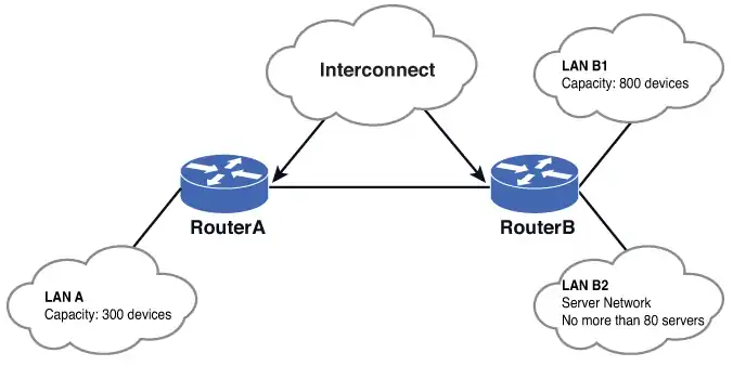
Solution:
For LAN A, a CIDR block that can handle at least 300 networking devices must be provided. In this case, two contiguous Class C networks of 192.168.0.0/24 and 192.168.1.0/24 can be grouped together to form a 192.168.0.0/23 network. Referring to Table 1-2, a /23 CIDR with a subnet mask of 255.255.254.0 provides 512 IP addresses which more than satisfies the required 300 networking devices.
The next question is to determine what the network address is for LAN A. This can be determined by ANDing the 255.255.254.0 subnet mask with 192.168.0.0 and 192.168.1.0.
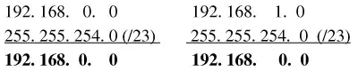
This shows that applying the /23 [255.255.254.0] subnet mask to the specified IP address places both in the same 192.168.0.0 network. This also means that this CIDR block does not cross boundaries, because applying the subnet mask to each network address places both in the same 192.168.0.0 network.
For LAN B1, the requirement is that a CIDR block that can handle 800 network devices must be provided. According to Table 1-2, a /22 CIDR yields 1,022 usable host IP addresses and is equivalent to grouping four Class C networks together. Therefore, a /22 CIDR can be used.
The next decision is selecting the group of IP addresses to create the CIDR block and decide where the IP addresses should start. Recall that the 192.168.0.0 and 192.168.1.0 networks are being used to create the LAN A CIDR block. Should LAN B1 start from 192.168.2.0/22, which is the next contiguous space? The answer is no. The 192.168.2.0/22 is still within the boundary of the 192.168.0.0/23 network.
Remember, the requirement is that a CIDR block that can handle 800 network devices must be provided and that boundaries cannot be crossed, and the designer must be careful not to overlap the networks when assigning subnets to more than one network. In this case, when the /22 subnet mask (255.255.252.0) is applied to 192.168.2.0, this yields the network 192.168.0.0.
The AND operation is shown:
192. 168. 2. 0
255. 255.252. 0 (/22)
192. 168. 0. 0
This happens to be the same network address as when the /23 CIDR subnet mask (255.255.254.0) is applied to any IP within the range of 192.168.0.0-192.168.1.255, as shown:
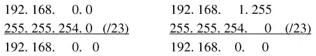
There is an overlap between 192.168.0.0/23 and 192.168.2.0/22. Moving to the next contiguous Class C of 192.168.3.0/22, we still find that it’s still in the 192.168.0.0:
192.168.3.0
255.255.252.0 (/22)
192.168.0.0 is still in the same subnet.
Based on this information, the next Class C range 192.168.4.0/22 is selected. This yields a nonoverlapping network of 192.168.4.0, so the subnet 192.168.4.0/22 is a valid for this network:
192.168.4.0
255.255.252.0 (/22)
192.168.4.0 is not the same subnet; therefore, this is an acceptable CIDR block.
Recall that the CIDR for LANB1 is a /22 and is equivalent to grouping four Class C networks.
This means that LANB1 uses the following Class C networks:
- 192.168.4.0
- 192.168.5.0
- 192.168.6.0
- 192.168.7.0
The IP subnet design gets more complicated when designing multiple networks with different size subnets. This usually means that the subnet mask or the CIDR will not be uniformly assigned to every network. For example, one network might be a /25 network or /22, while another is a /30 network.
The next requirement is that a CIDR block that can handle 800 network devices must be tasked to assign a CIDR block to LAN B2. This LAN is a server network that houses a fixed number of servers. The number is not expected to grow beyond 80 servers. One easy approach is to assign a /24 CIDR to this network.
This means that the next network is 192.168.8.0/24, which is the next nonoverlapping CIDR block after 192.168.4.0/22. The /24 CIDR gives 254 host IP addresses, but only 80 IP addresses are required. Another approach is to size it appropriately. According to Table 2 (above), a good CIDR to use is a /25, which allows for 126 host IP addresses. Therefore, a network 192.168.8.0/25 can be used for this network.
Assigning a 192.168.8.0/24 CIDR, which can accommodate 254 hosts, seems like a waste, because the network is expected to be a fixed size, and it will house no more than 80 servers. By assigning a 192.168.8.0/25 CIDR, enough room is left for another contiguous CIDR, 192.168.8.128/25. Obviously, this is a more efficient way of managing the available IP space.
Last but not least is the interconnection shown in Image 4 (above, in example 1). This is the router-to-router link between Router A and Router B. The interconnection usually gets the least attention, but it exists everywhere in the multiple network environment. Nonetheless, a CIDR block has to be assigned to it. Because there are always only two interface IP addresses involved plus the network and broadcast address, giving an entire Class C address would definitely be a waste. Typically, a /30 CIDR is used for this type of connection.
Therefore, a CIDR block for the interconnection between Router A and Router B can be 192.168.9.0/30. This yields two IP host addresses: one for Router A and one for Router B.
The complete subnet assignment for Example 1 and Image 4 is provided in Table 3.
| Network | Subnet | CIDR | Subnet Mask |
| LAN A | 192.168.0.0 | /23 | 255.255.254.0 |
| LAN B1 | 192.168.4.0 | /22 | 255.255.252.0 |
| LAN B2 | 192.168.8.0 | /24 or /25 | 255.255.255.0 or 255.255.255.128 |
| Interconnect | 192.168.9.0 | /30 | 255.255.255.252 |
IP Assignment
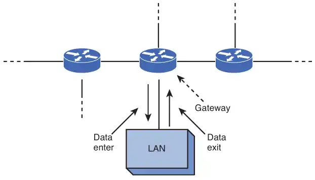
The next task requirement is that a CIDR block that can handle 800 network devices must be required to assign an IP address to each routed interface. This address will become the gateway IP address of the subnet. The gateway describes the networking device that enables hosts in a LAN to connect to networks (and hosts) outside the LAN. Image 5 provides an example of the gateway.
Every network device within its subnet (LAN) will use this IP address as its gateway to communicate from its local subnet to devices on other subnets. The gateway IP address is preselected and is distributed to a network device by way of manual configuration or dynamic assignment.
For LAN A in Example 1, the IP address 192.168.0.0 is already reserved as the network address, and the IP address 192.168.0.255 is reserved as the broadcast address. This leaves any IP address within the range 192.168.0.1–192.168.0.254 available for use for the gateway address. Choosing the gateway IP address is not an exact science.
Normally, the first IP address or the last IP address of the available range is chosen. Whatever convention is chosen, it should apply to the rest of the subnets for the ease of management. Once the gateway IP address is chosen, this IP address is reserved and is not to be used by any other devices in the subnet. Otherwise, an IP conflict will be introduced. The following is an example of how the gateway IP addresses could be assigned to the LANs in Example 1.
| Network | Gateway |
| LAN A | 192.168.0.1 |
| LAN B1 | 192.168.4.1 |
| LAN B2 | 192.168.8.1 |
VLAN Network
LANs are not necessarily restricted in size. A LAN can have 20 computers, 200 computers, or even more. Multiple LANs also can be interconnected to essentially create one large LAN. For example, the first floor of a building could be set up as one LAN, the second floor as another LAN, and the third floor another. The three LANs in the building can be interconnected into essentially one large LAN using switches, with the switches interconnected, as shown in Image 6.
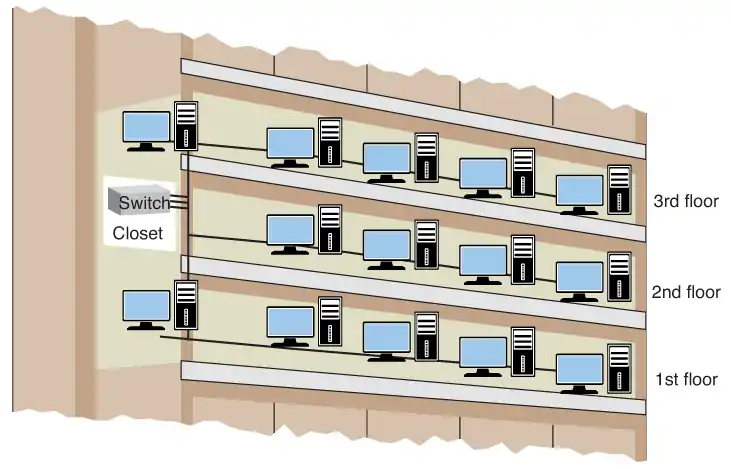
Is it bad to interconnect LANs this way?
As long as switches are being used to interconnect the computers, the interconnected LANs have minimal impact on network performance. This is true as long as there are not too many computers in the LAN. The number of computers in the LAN is an issue, because Layer 2 switches do not separate broadcast domains.
This means that any broadcast sent out on the network (for example, the broadcast associated with an ARP request) will be sent to all computers in the LAN. Excessive broadcasts are a problem, because each computer must process the broadcast to determine whether it needs to respond; this essentially slows down the computer and the network.
A network with multiple LANs interconnected at the Layer 2 level is called a flat network. A flat network is where the LANs share the same broadcast domain. The use of a flat network should be avoided, if possible, for the simple reason that the network response time is greatly affected.
Flat networks can be avoided by the use of virtual LANs (VLAN) or routers. Although both options can be used to separate broadcast domains, they differ in that the VLAN operates at the OSI Layer 2, while routers use Layer 3 networking to accomplish the task. The topic of a virtual VLAN is discussed next.
Virtual LAN (VLAN)
Obviously, if the LANs are not connected, then each LAN is segregated only to a switch. The broadcast domain is contained to that switch; however, this does not scale in a practical network, and it is not cost effective because each LAN requires its own Layer 2 switches. This is where the concept of virtual LAN (VLAN) can help out.
A VLAN is a way to have multiple LANs co-exist in the same Layer 2 switch, but their traffic is segregated from each other. Even though they reside on the same physical switch, they behave as if they are on different switches (hence, the term virtual). VLAN compatible switches can communicate to each other and extend the segregation of multiple LANs throughout the entire switched network.
A switch can be configured with a VLAN where a group of host computers and servers are configured as if they are in the same LAN, even if they reside across routers in separate LANs. Each VLAN has its own broadcast domain. Hence, traffic from one VLAN cannot pass to another VLAN. The advantage of using VLANs is the network administrator can group computers and servers in the same VLAN based on the organizational group (such as Sales, Engineering) even if they are not on the same physical segment—or even the same building.
There are three types of VLANs: port-based VLANs, tag-based VLANs, and protocol-based VLANs.
Port-based VLAN
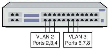
The port-based VLAN is one where the host computers connected to specific ports on a switch are assigned to a specific VLAN. For example, assume the computers connected to switch ports 2, 3, and 4 are assigned to the Sales VLAN 2, while the computers connected to switch ports 6, 7, and 8 are assigned to the Engineering VLAN 3, as shown in Image 7. The switch will be configured as a port-based VLAN so that the groups of ports [2,3,4] are assigned to the sales VLAN while ports [6,7,8] belong to the Engineering VLAN.
The devices assigned to the same VLAN will share broadcasts for that LAN; however, computers that are connected to ports not assigned to the VLAN will not share the broadcasts. For example, the computers in VLAN 2 (Sales) share the same broadcast domain and computers in VLAN 3 (Engineering) share a different broadcast domain.
Tag-based VLAN
In tag-based VLANs, a tag is added to the Ethernet frames. This tag contains the VLAN ID that is used to identify that a frame belongs to a specific VLAN. The addition of the VLAN ID is based on the 802.1Q specification. The 802.1Q standard defines a system of VLAN tagging for Ethernet frames. An advantage of an 802.1Q VLAN is that it helps contain broadcast and multicast data traffic, which helps minimize data congestion and improve throughput. This specification also provides guidelines for a switch port to belong to more than one VLAN. Additionally, the tag-based VLANs can help provide better security by logically isolating and grouping users.
Protocol-based VLAN
In protocol-based VLANs, the data traffic is connected to specific ports based on the type of protocol being used. The packet is dropped when it enters the switch if the protocol doesn’t match any of the VLANs. For example, an IP network could be set up for the Engineering VLAN on ports 6,7,8 and an IPX network for the Sales VLAN on ports 2,3, and 4. The advantage of this is the data traffic for the two networks is separated.
There are two approaches for assigning VLAN membership:
• Static VLAN: Basically, a port-based VLAN. The assignments are created when ports are assigned to a specific VLAN.
• Dynamic VLAN: Ports are assigned to a VLAN based on either the computer’s MAC address or the username of the client logged onto the computer. This means that the system has been previously configured with the VLAN assignments for the computer or the username. The advantage of this is the username and/or the computer can move to a different location, but VLAN membership will be retained.
Routed Network
This section examines the Layer 3 network and how data is routed in the network. This section also introduces another Layer 3 device, the multilayer switch. You need to understand the advantages and disadvantages of this device. This section also introduces interVLAN configuration, which enables VLANs to communicate across networks. The section concludes with a look at both serial and ATM configurations. Some network engineers will argue that the serial and ATM technologies are a dying technology and are now considered obsolete. However, being obsolete does not mean they are nonexistent. These technologies are still being used throughout the world, and it is still an important topic.
Router
The router is a powerful networking device used to interconnect LANs. The router is a Layer 3 device in the OSI model, which means the router uses the network address (Layer 3 addressing) to make routing decisions regarding forwarding data packets. In the OSI model, the Layer 3, or network, layer responsibilities include handling of the network address. The network address is also called a logical address, rather than being a physical address (such as the MAC address, which is embedded into the network interface card [NIC]). The logical address describes the IP address location of the network and the address location of the host in the network.
Essentially, the router is configured to know how to route data packets entering or exiting the LAN. This differs from the bridge and the Layer 2 switch, which use the Ethernet address for making decisions regarding forwarding data packets and only know how to forward data to hosts physically connected to their ports.
Routers are used to interconnect LANs in a campus network. Routers can be used to interconnect networks that use the same protocol (for example, Ethernet), or they can be used to interconnect LANs that are using different Layer 2 technologies, such as an Ethernet, ATM, T1, and so on. Routers also make it possible to interconnect to LANs around the country and the world and interconnect to many different networking protocols.
The router ports are bidirectional, meaning that data can enter and exit the same router port. Often, the router ports are called the router interface, which is the physical connection where the router connects to the network.
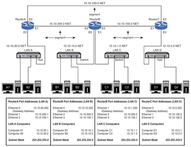
The network provided in Image 8 is an example of a simple three-router campus network. This configuration enables data packets to be sent and received from any host on the network after the routers in the network have been properly configured. For example, computer A1 in LAN A could be sending data to computer D1 in LAN D. This requires that the IP address for computer D1 is known by the user sending the data from computer A1.
The data from computer A1 will first travel to the switch where the data is passed to Router A via the FA0/0 FastEthernet data port. Router A will examine the network address of the data packet and use configured routing instructions stored in the router’s routing tables to decide where to forward the data.
Router A determines that an available path to Router C is via the FA0/2 FastEthernet port connection. The data is then sent directly to Router C. Router C determines that the data packet should be forwarded to its FA0/0 port to reach computer D1 in LAN D. The data is then sent to D1. Alternatively, Router A could have sent the data to Router C through Router B via Router A’s FA0/1 FastEthernet port.
Delivery of the information over the network was made possible by the use of an IP address and routing table. Routing tables keep track of the routes used for forwarding data to its destination. Router A used its routing table to determine a network data path so computer A1’s data could reach computer D1 in LAN D.
After the data packet arrived on Router C, an ARP request is issued by Router C to determine the MAC address of computer D1. The MAC address is then used for final delivery of the data to computer D1.
If Router A determines that the network path to Router C is down, Router A can route the data packet to Router C through Router B. After Router B receives the data packet from Router A, it uses its routing tables to determine where to forward the data packet. Router B determines that the data needs to be sent to Router C. Router B will then use its FA0/3 Fast Ethernet port to forward the data to Router C.
Gateway Address
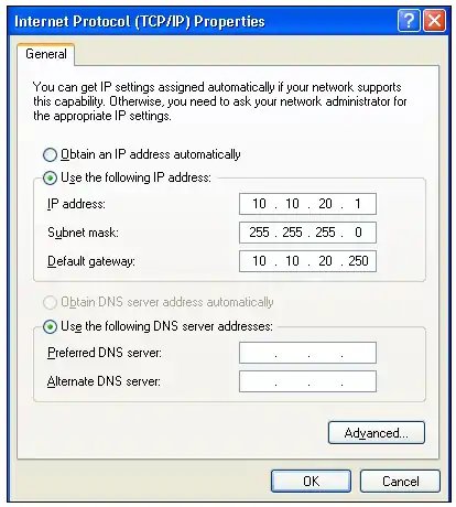
As previously discussed, the term gateway is used to describe the address of the networking device that enables the hosts in a LAN to connect to networks and hosts outside the LAN. For example, the gateway address for all hosts in LAN A will be 10.10.20.250. This address is configured on the host computer, as shown in Image 9. Any IP packets with a destination outside the LAN A network will be sent to this gateway address. Note that the destination network is determined by the subnet mask. In this case, the subnet mask is 255.255.255.0.
Network Segments
The network segment defines the networking link between two LANs. There is a segment associated with each connection of an internetworking device (for example, router-hub, router-switch, router-router). For example, the IP address for the network segment connecting LAN A to the router is 10.10.20.0. All hosts connected to this segment must contain a 10.10.20.x, because a subnet mask of 255.255.255.0 is being used. Subnet masking is fully explained in Network Essentials Chapter 6, “TCP/IP.”
Routers use the information about the network segments to determine where to forward data packets. For example, referring to Image 8, the network segments that connect to Router A include
- 10.10.20.0
- 10.10.200.0
- 10.10.100.0
The segment is sometimes called the subnet or NET. These terms are associated with a network segment address, such as 10.10.20.0. In this case, the network is called the 10.10.20.0 NET. All hosts in the 10.10.20.0 NET will have a 10.10.20.x IP address. The network addresses are used when configuring the routers and defining which networks are connected to the router.
According to Image 9, all the computers in LAN A must have a 10.10.20.x address. This is defined by the 255.255.255.0 subnet mask. For example, computer A1 in LAN A will have the assigned IP address of 10.10.20.1 and a gateway address of 10.10.20.250. The computers in LAN B (see Image 8) are located in the 10.10.10.0 network. This means that all the computers in this network must contain a 10.10.10.x IP address.
In this case, the x part of the IP address is assigned for each host. The gateway address for the hosts in LAN B is 10.10.10.250. Notice that the routers are all using the same .250 gateway address. Remember, any valid IP address can be used for the gateway address, but it is a good design procedure to use the same number for number for all routers. In this case, .250 is being used. In other cases, it could be .1 or .254.
The subnet mask is used to determine whether the data is to stay in the LAN or is to be forwarded to the default gateway provided by the router. The router uses its subnet mask to determine the destination network address. The destination network address is checked with the router’s routing table to select the best route to the destination. The data is then forwarded to the next router, which is the next hop address.
The next router examines the data packet, determines the destination network address, checks its routing table, and then forwards the data to the next hop. If the destination network is directly connected to the router, it issues an ARP request to determine the MAC address of the destination host. Final delivery is then accomplished by forwarding the data using the destination host computer’s MAC address. Routing of the data through the networks is at Layer 3, and the final delivery of data in the network is at Layer 2.
Multilayer Switch
So far, the topic of network switches revolves around their Layer 2 functionalities. Today, the scope of operations has changed for switches. Newer switch technologies are available to help further improve the performance of computer networks. This new development started with Layer 3 switches and now there are multilayer switches. The term used to describe these switches that can operate above the OSI Layer 2 is multilayer switches (MLS).
An example is a Layer 3 switch. Layer 3 switches still work at Layer 2, but additionally work at the network layer (Layer 3) of the OSI model and use IP addressing for making decisions to route a data packet in the best direction. The major difference is that the packet switching in basic routers is handled by a programmed microprocessor. The multilayer switch uses application specific integrated circuits (ASIC) hardware to handle the packet switching.
The advantage of using hardware to handle the packet switching is a significant reduction in processing time (software versus hardware). In fact, the processing time of multilayer switches can be as fast as the input data rate. This is called wire speed routing, where the data packets are processed as fast as they are arriving. Multilayer switches can also work at the upper layers of the OSI model. An example is a Layer 4 switch that processes data packets at the transport layer of the OSI model.
Through this evolution, the line between routers and multilayer switches is getting more and more blurry. Routers were once considered the more intelligent device, but this is no longer true. With new developments, the multilayer switches can do almost everything the routers can. More importantly, most of the Layer 3 switch configuration commands are almost identical to the ones used on the routers. Routers tend to be more expensive when it comes to cost per port. Therefore, most of the traditional designs have a router connecting to a switch or switches to provide more port density. This can be expensive depending on the size of the network.
So, there has been a shift toward deploying multilayer switches in the network LAN environment in place of routers. In this case, the routers and switches in Image 8 then could all be replaced with multilayer switches. This also means there will be less network equipment to maintain, which reduces the maintenance cost and makes this a more cost-effective solution. With its greater port density, a multilayer switch can serve more clients than a router could. However, there is a common drawback for most multilayer switches: These devices only support Ethernet. Other Layer 2 technologies, such as ATM, DSL, T1, still depend on routers for making this connection.
Layer 3 Routed Networks
As discussed previously, the hosts are interconnected with a switch or hub. This allows data to be exchanged within the LAN; however, data cannot be routed to other networks. Also, the broadcast domain of one LAN is not isolated from another LAN’s broadcast domain. The solution for breaking up the broadcast domains and providing network routing is to incorporate routing hardware into the network design to create a routed network. A routed network uses Layer 3 addressing for selecting routes to forward data packets, so a better name for this network is a Layer 3 network.
In Layer 3 networks, routers and multilayer switches are used to interconnect the networks and LANs, isolating broadcast domains and enabling hosts from different LANs and networks to exchange data. Data packet delivery is achieved by handing off data to adjacent routers until the packet reaches its final destination. This typically involves passing data packets through many routers and many networks. An example of a Layer 3 network is shown in Image 8. This example has four LANs interconnected using three routers. The IP address for each networking device is listed.
The physical layer interface on the router provides a way to connect the router to other networking devices on the network. For example, the FastEthernet ports on the router are used to connect to other FastEthernet ports on other routers or switches. Gigabit and 10-gigabit Ethernet ports are also available on routers to connect to other high-speed Ethernet ports (the sample network shown in Image 8 includes only FastEthernet ports). Routers also contain other types of interfaces, such as serial interfaces and Synchronous Optical Network (SONET) interfaces.
These interfaces were widely used to interconnect the router and the network to other wide-area networks (WAN). For example, connection to WANs requires the use of a serial interface or SONET interface to connect to a communications carrier, such as Sprint, AT&T, Century Link, and so on. The data speeds for the serial communication ports on routers can vary from slow (56 kbps) up to high-speed DS3 data rates (47+ Mbps), and the SONET could range from OC3 (155 Mbps), OC12 (622 Mbps), or even OC192 (9953 Mbps).
If you want to learn more about network infrastructure design please take a look at this book: A Practical Guide to Advanced Networking, Jeffrey S. Beasley and Piyasat Nilkaew, 2012. You can find it on Amazon.